Pay Attention, Relations are Important

Overview
In recent years, Knowledge Graphs have been utilized to solve many real world problems such as Semantic Search, Dialogue Generation and Question Answering to name a few. Knowledge Graphs suffer from incompleteness in form of missing entities and relations, which has fueled a lot of research on Knowledge Base completion. Relation prediction is one of the widely used approaches to solve the problem of incompleteness.
Here we will present our ACL 2019 work, Learning Attention-based Embeddings for Relation Prediction in Knowledge Graphs, and introduce a novel neural network architecture which operates on Knowledge Graphs and learns to extract more expressive feature representations for entities and relations. Our model also addresses the shortcomings of previous methods like ConvKB, ConvE, RGCN, TransE, DistMult and ComplEx.
The code for this publication is provided here. We will discuss how to reproduce the results given in the paper at the end of this post.
Graph Convolution Networks
Convolutional Neural Networks (CNNs) have helped in significantly improving the state-of-the-art in Computer Vision research. Image data can be seen as a spatial grid which is highly rigid (each pixel is connected to it’s 8 neighboring pixels). The CNNs exploit the rigidity and regular connectivity pattern of image data and thus give us an effective and trivial method to implement convolution operator.
Convolution operator in images gathers information from neighboring pixels commensurately. Similar idea is used when defining convolution operation on graphs.
Now Consider, a graph with \(n\) nodes, specified as set of node features \(\textbf{x} = \{\vec{x}_{1},\vec{x}_{2},...,\vec{x}_{N}\}\) and the connectivity information in form of adjacency matrix \(A\). A graph convolutional layer then produces a transformed set of node feature vectors \(\textbf{x}^\prime = \{\vec{x}_{1}^{\prime},\vec{x}_{2}^{\prime},...,\vec{x}_{N}^{\prime}\}\) based on the structure of the graph and intial embeddings of the entities.
The convolution operation on graph can be summarized with the help of following two operations. First, in order to achieve a higher order representation of nodes, we do a linear transformation parametrized by a weight matrix \(\textbf{W}\). The transformed feature vectors \(\vec{g_{i}}\) are given as \(\vec{g_{i}} = \textbf{W}\vec{x_{i}}\). Finally, to get the output features of node \(i\), we will aggregate the features across the neighborhood of the node. Final feature vectors \(\vec{x^{'}_{i}}\) can be defined as:
\[\begin{aligned} \vec{x_{i}^{\prime}} = \sigma \Bigg( \sum_{j \in \mathcal{N}_{i}} \alpha_{ij} \vec{g_{j}} \Bigg) \end{aligned}\]where \(\sigma\) is an activation function, \(\mathcal{N}_{i}\) defines the neighborhood of node \(i\), and \(\alpha_{ij}\) specifies the importance of node \(j^{'}s\) features to node \(i\).
In most of the prior works, \(\alpha_{ij}\) is defined explicitly, based on structural properties or as a learnable weight.
Graph Attention Networks
We just saw how graph convolution works for arbitrary graph. Vaswani et al., 2017 It has been shown that self-attention can help us go above and beyond on the task of machine translation, Vaswani et al 2017(Transformer). Taking motivation from the previous success of self-attention mechanism, the GAT(cite) defines the value of \(\alpha_{ij}\) implicitly.
Computation of \(\alpha_{ij}\) is a result of an attentional mechanism \(a\) applied over node features. The un-normalized attention coefficients over node pair \(i,j\) are computed as follows:
\[e_{ij} = a(\vec{g}_{i}, \vec{g}_{j})\]where \(\vec{g}_i\) and \(\vec{g}_{j}\) are transformed feature vectors of nodes \(i\) and \(j\), as described in previous section.
The node \(i\) is allowed to attend over it’s neighborhood, \(j \in \mathcal{N}_{i}\). These un-normalized attention values cannot be used to compare the importance of different nodes, so typically the coefficients are normalized by using a softmax function. The final output of a Graph Attention Layer is calculated by gathering the information from the neighborhood as shown in the following equation:
\[\vec{x_{i}^{\prime}} = \sigma \Bigg( \sum_{j \in \mathcal{N}_{i}} \alpha_{ij} \textbf{W} \vec{x_{j}} \Bigg)\]Multi-head attention mechanism is employed to stabilize the learning process, taking the motivation from Vaswani et al, 2017. The above operations are independently applied to the node features and the outputs are featurewise aggregated, by concatenating or by adding (as is the case in last layer).
\[\vec{x_{i}^{\prime}} = \underset{k=1}{\stackrel{K}{\Big \Vert}} \sigma \Bigg( \sum_{j \in \mathcal{N}_{i}} \alpha_{ij}^{k} \textbf{W}^{k} \vec{x_{j}} \Bigg)\]where \(\Vert\) represents concatenation, \(\sigma\) represents any non-linear activation function, \(\alpha_{ij}^{k}\) are normalized attention coefficients calculated by the \(k\)-th attention mechanism, and \(\textbf{W}^k\) represents the corresponding linear transformation matrix of the \(k\)-th attention mechanism.This fully specifies a Graph Attention Layer!
Now we can work with arbitrary structured graphs, Good! But, what about Knowledge Graphs, are GATs good enough to produce best results on those kind of graphs? How are Knowledge Graphs different? We discuss this in the next section and give a novel architecture to tackle some of the shortcomings of existing method.
Brief introduction to Knowledge graphs Embeddings
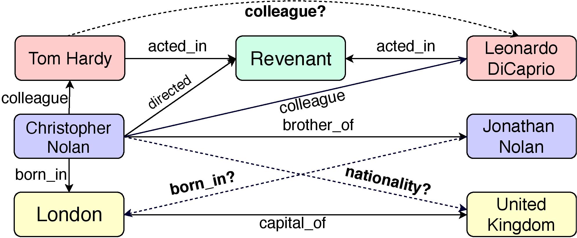
A knowledge graph is denoted by \(\mathcal{G}=(\mathcal{E}, R)\), where \(\mathcal{E}\) and \(R\) represent the set of entities (nodes) and relations (edges), respectively. A triple \((e_s, r, e_o)\) is represented as an edge \(r\) between nodes \(e_s\) and \(e_r\) in \(\mathcal{G}\). A triple in the Knowledge Graph denotes a fact, for example in the image, the triple (London, capital_of, United Kingdom) represents the fact that London is the capital of United Kingdon, so capital_of is the relatoin between two specified entities.

Embedding models try to learn an effective representation of entities, relations, and a scoring function \(f\), such that for a given input triple \(t = (e_s, r, e_o)\), \(f(t)\) gives the likelihood of \(t\) being a valid triple. For example, above figure shows the subgraph from a KG which infers missing links represented by dashed lines using existing triples such as (London, captial_of, United Kingdom).
It is the relations between entities that differentiates the Knowledge Graphs from other types of graphs. As can be understood by observing the structure of Knowledge Graphs, relations are an integral part of these graphs. An entity can play multiple roles depending on the relation by which they are connected. For example, in the above figure, Christopher Nolan plays different roles of brother and a director. Thus, while working with Knowledge Graphs, it’s just not enough to focus on entities and ignore relations!
KBAT (Knowledge Base Attention) Network
With the preceding information as our motivation, we define a novel neural network architecture, Knowledge Base Attention Network, which uses the self-attention mechanism to attend over the neighborhood of every node and takes into account the relations in the Knowledge Graphs.
Consider a Knowledge Graph \(\mathcal{G}\), with Entity embedding matrix \(\textbf{H} \in \mathbb{R}^{N_e \times T}\), where the \(i\)-th row is the embedding of entity \(e_i\), \(N_e\) is the total number of entities, and \(T\) is the feature dimension of each entity embedding. With a similar construction, the relation embeddings are represented by a matrix \(\textbf{G} \in \mathbb{R}^{N_r \times P}\). Taking these two embedding matrices as input, the layer outputs the corresponding embedding matrices, \(\textbf{H}^\prime \in \mathbb{R}^{N_e \times T^\prime}\) and \(\textbf{G}^\prime \in \mathbb{R}^{N_r \times P^\prime}\). We define an edge tuple \(t_{ij}^{k}\) as, \(t_{ij}^{k} = (e_i, r_k, e_j)\), where \(e_i, e_j\) are the entities and \(r_k\) is the relation joining these two entities.
To incorporate the relations, we learn a new representation of every edge and aggregate the information by summing this over the neighborhood multiplying with the appropriate attention values. We learn these embeddings by performing a linear transformation over the concatenation of entity and relation feature vectors corresponding to a particular triple \(t_{ij}^{k} = (e_i, r_k, e_j)\) as shown:
\[\vec{c_{ijk}} = \textbf{W}_{1} [\vec{h}_{i} \Vert \vec{h}_{j} \Vert \vec{g}_{k}]\]where \(\vec{c_{ijk} }\) is the vector representation of a triple \(t_{ij}^k\). Vectors \(\vec{h}_i, \vec{h}_j\), and \(\vec{g}_k\) denote embeddings of entities \(e_i, e_j\) and relation \(r_k\), respectively. Additionally, \(\textbf{W}_1\) denotes the linear transformation matrix.
We use a self-attention mechanism \(a\), to compute the un-normalized attention coefficients \(b_{ijk}\), for all edge tuple \(t_{ij}^k\) for all the tuples in the neighborhood \(\mathcal{N_i}\) of node \(i\):
\[b_{ijk} = a(\vec{h}_{i}, \vec{g}_k, \vec{h}_{j})\]where \(\vec{h}_i, \vec{h}_j\) denote the embeddings of \(i^{th}\) and \(j^{th}\) entities.
The framework is agnostic to the attention mechanism \(a\). In this work, we use a single layered neural network as an attention mechanism and the calculation is shown in the equation below:
\[b_{ijk} = \textrm{LeakyReLU} \Big( \textbf{W}_{2} c_{ijk} \Big)\]where \(\textbf{W}_2\) is the linear transformation matrix.
Similar to the GAT layer, we use the softmax function to normalize these attention values to be useful across the neighborhoods and the normalized attention values \(\alpha_{ijk}\) are calculated:
\[\alpha_{ijk} = \frac{\textrm{exp} (b_{ijk})}{\sum_{n \in \mathcal{N}_{i}} \sum_{r \in \mathcal{R}_{in}} \textrm{exp} (b_{inr})}\]where \(\mathcal{N}_i\) denotes the neighborhood of entity \(e_i\) and \(\mathcal{R}_{ij}\) denotes the set of relations connecting entities \(e_i\) and \(e_j\).
The new embedding of the entity \(e_i\) is calculated by aggregating the information from the neighborhood by summing each triple representation weighted by their attention values as shown:
\[\vec{h_{i}^{\prime}} = \sigma \Bigg( \sum_{j \in \mathcal{N}_{i}} \sum_{k \in \mathcal{R}_{ij}} \alpha_{ijk} \vec{c_{ijk}} \Bigg)\]We employ a similar multi-head attention mechanism to GAT, which was first introduced by Vaswani et al., 2017 , is used to stabilize the learning process and encapsulate more information about the neighborhood.
\[\vec{h_{i}^{\prime}} = \underset{m=1}{\stackrel{M}{\Big \Vert}} \sigma \Bigg( \sum_{j \in \mathcal{N}_{i}} \alpha_{ijk}^{m} c_{ijk}^{m} \Bigg)\]We perform a linear transformation on input relation embedding matrix \(\textbf{G}\), and get the transformed relation embeddings \(G^\prime \in \mathbb{R}^{N_r \times T^\prime}\), where \(T^\prime\) is shared output dimensionality of entity and relation embeddings.
\[G^{\prime} = G.\textbf{W}^{R}\]In the Graph Convolution and Graph Attention Networks, its a good practice to add a self loop to every entity so that the information of that entity also plays a role in it’s new embeddings. However, if we cannot do the same in Knowledge graphs because adding a self loop means adding a new relation type which does not makes sense. On the other hand, ignoring the previous information stored in the embeddings doesn’t seem like a good idea. We resolve this issue by linearly transforming \(\textbf{H}^i\) to obtain \(\textbf{H}^t\) using a weight matrix \(\textbf{W}^E \in \mathbb{R}^{T^i \times T^f}\), where \(\textbf{H}^i\) represents the input entity embeddings to our model, \(\textbf{H}^t\) represents the transformed entity embeddings, \(T^i\) denotes the dimension of an initial entity embedding, and \(T^f\) denotes the dimension of the final entity embedding. We add this initial entity embedding information to the entity embeddings obtained from the final attentional layer, \(\textbf{H}^f \in \mathbb{R}^{N_e \times T^f}\) as shown below:
\[\textbf{H}^{\prime\prime} = \textbf{W}^E \textbf{H}^t + \textbf{H}^{f}\]With this preceding information, we have succefully defined a Knowledge Base Attention Layer!
Auxiliary Edges
In our architecture, we extend the notion of an edge to a directed path by introducing an auxiliary relation for \(n\)-hop neighbors between two entities. In the current mode, the embedding of this auxiliary relation is the featurewise summation of embeddings of all the relations in the path. However, the summation operation can be replaced with a max pooling operation.

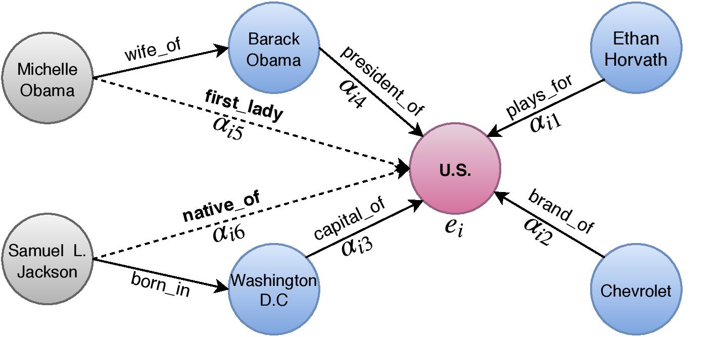
Let’s see an easy example how KBAT works. KBAT iteratively accumulates knowledge from distant neighbors of an entity. As illustrated in the image above, in the first layer of this model, all entities capture information from their direct in-flowing neighbors. In the second layer, U.S gathers information from entities Barack Obama, Ethan Horvath, Chevrolet, and Washington D.C, which already possess information about their neighbors Michelle Obama and Samuel L. Jackson, from a previous layer. In general, for a \(n\) layer model the incoming information is accumulated over a \(n\)-hop neighborhood. We found that normalizing the entity embeddings after every generalized KBAT layer and prior to the first layer was useful.
Is that enough?
We used a decoder network to decode the information collected by KBAT and use that decoded information for the ranking task. We used ConvKB as a decoder model. And we found that while KBAT networks does a good job at collecting information from the neighborhood, that information can not be directly used to make amazing predictions. This concludes the explanation of our model, KBAT (The Encoder) and a decoder network (ConvKB in this case).
Reproducing the results
In this section we will first summarize how to use KBAT model on new datasets (not available in our github repo). Once we are done with the basic setup and initialization, there will be steps on reproducing the results given in the paper.
- Let’s start with cloning the github repository which contains pytorch implementation of KBAT network.
$ git clone https://github.com/deepakn97/relationPrediction.git - If you wish to reuse the dataset provided please feel free to skip to step 4. Now we need to create a new data directory and populate the directory with some important files.
- entity2id.txt: contains mapping of entity names to the id. id starts from 0.
- relation2id.txt: contains mapping of relation names to the id. id starts from 0.
- train.txt and test.txt: contains list of triples in the format entity1 relation entity2 For better example, please inspect one of the data directories.
- KBAT network requires to initialize the entity and relation embedding vectors before it can start training. We use TransE embeddings to initialize these vectors. Set of commands given below can be used to get embedding files. For more detailed information please refer here.
    $ git clone https://github.com/datquocnguyen/STransE.git
    $ cd ./SOURCE_DIR
    SOURCE_DIR$ g++ -I ../SOURCE_DIR/ STransE.cpp -o STransE -O2 -fopenmp -lpthread
    SOURCE DIR$ /STransE -model 1_OR_0 -data CORPUS_DIR_PATH -size <int> -l1 1_OR_0 -margin <double> -lrate <double>
- Now we have everything in place and we can start training the model. Once the training completes, the model will automatically evaluate it’s performance on the given test set. To train the model we need to run main.py using the following command.
$ python3 main.py -data [data_dir]
To find about all the parameters available please look at the github repository. We also provide a values of all the parameters used for producing the results reported in the paper.
Citation
Please cite the following paper if you use this code in your work.
    @InProceedings{KBGAT2019,
    author = "Nathani, Deepak and Chauhan, Jatin and Sharma, Charu and Kaul, Manohar",
    title = "Learning Attention-based Embeddings for Relation Prediction in Knowledge Graphs",
    booktitle = "Proceedings of the 57th Annual Meeting of the Association for Computational Linguistics",
    year = "2019",
    publisher = "Association for Computational Linguistics",
    location = "Florence, Italy",
    }
For any query or suggestion, please drop a mail at deepakn1019@gmail.com.